Unsupervised Learning cheatsheet
By Afshine Amidi and Shervine Amidi
Introduction to Unsupervised Learning
- Motivation: The goal of unsupervised learning is to find hidden patterns in unlabeled data \(\{x^{(1)},...,x^{(m)}\}\).
- Jensen's inequality: Let \(f\) be a convex function and \(X\) a random variable. We have the following inequality:
\[ \boxed{E[f(X)]\geqslant f(E[X])} \]
Clustering
Expectation-Maximization
- Latent variables: Latent variables are hidden/unobserved variables that make estimation problems difficult, and are often denoted \(z\). Here are the most common settings where there are latent variables:
| Setting | Mixture of \(k\) Gaussians | Factor analysis |
|---|---|---|
| Latent variable \(z\) | \(\textrm{Multinomial}(\phi)\) | \(\mathcal{N}(0,I)\) |
| \(x|z\) | \(\mathcal{N}(\mu_j,\Sigma_j)\) | \(\mu_j\in\mathbb{R}^n, \phi\in\mathbb{R}^k\) |
| Comments | \(\mathcal{N}(\mu+\Lambda z,\psi)\) | \(\mu_j\in\mathbb{R}^n\) |
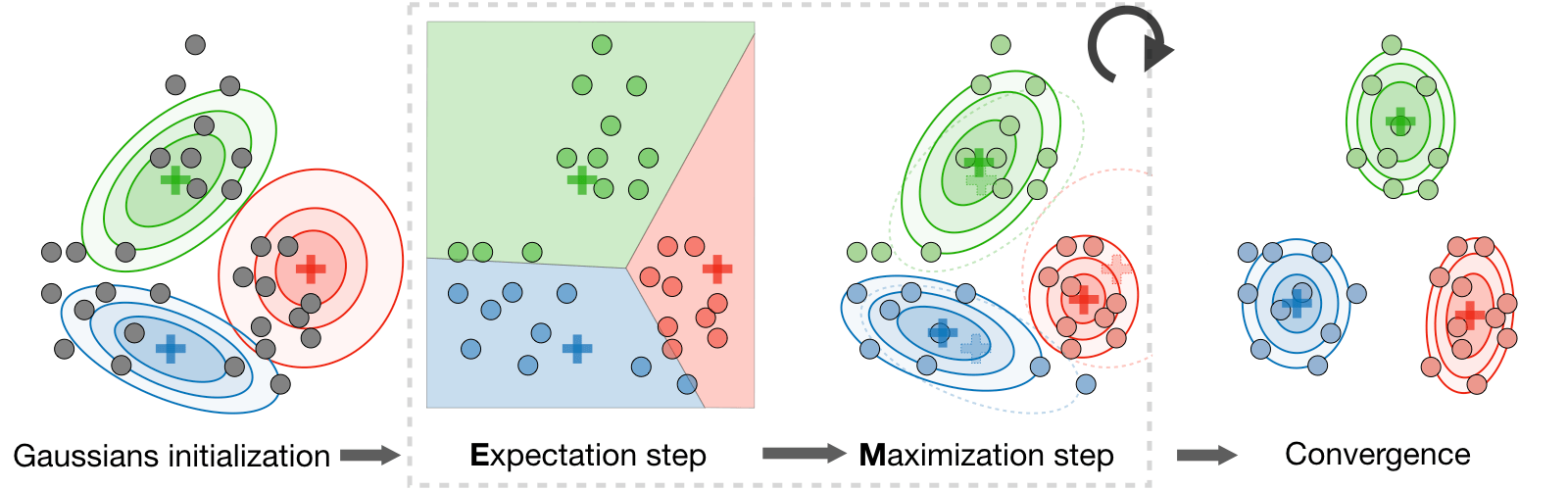
Algorithm: The Expectation-Maximization (EM) algorithm gives an efficient method at estimating the parameter \(\theta\) through maximum likelihood estimation by repeatedly constructing a lower-bound on the likelihood (E-step) and optimizing that lower bound (M-step) as follows:
E-step: Evaluate the posterior probability \(Q_{i}(z^{(i)})\) that each data point \(x^{(i)}\) came from a particular cluster \(z^{(i)}\) as follows:
\[ \boxed{Q_i(z^{(i)})=P(z^{(i)}|x^{(i)};\theta)} \]
M-step: Use the posterior probabilities \(Q_i(z^{(i)})\) as cluster specific weights on data points \(x^{(i)}\) to separately re-estimate each cluster model as follows:
\[ \boxed{\theta_i=\underset{\theta}{\textrm{argmax }}\sum_i\int_{z^{(i)}}Q_i(z^{(i)})\log\left(\frac{P(x^{(i)},z^{(i)};\theta)}{Q_i(z^{(i)})}\right)dz^{(i)}} \]
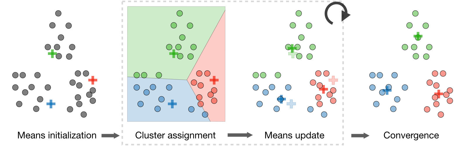
\(k\)-means clustering
We note \(c^{(i)}\) the cluster of data point \(i\) and \(\mu_j\) the center of cluster \(j\).
- Algorithm: After randomly initializing the cluster centroids \(\mu_1,\mu_2,...,\mu_k\in\mathbb{R}^n\), the \(k\)-means algorithm repeats the following step until convergence:
\[ \boxed{c^{(i)}=\underset{j}{\textrm{arg min}}\|x^{(i)}-\mu_j\|^2}\quad\textrm{and}\quad\boxed{\mu_j=\frac{\displaystyle\sum_{i=1}^m1_{\{c^{(i)}=j\}}x^{(i)}}{\displaystyle\sum_{i=1}^m1_{\{c^{(i)}=j\}}}} \]
- Distortion function: In order to see if the algorithm converges, we look at the distortion function defined as follows:
\[ \boxed{J(c,\mu)=\sum_{i=1}^m\|x^{(i)}-\mu_{c^{(i)}}\|^2} \]
Hierarchical clustering
- Algorithm: It is a clustering algorithm with an agglomerative hierarchical approach that build nested clusters in a successive manner.
- Types: There are different sorts of hierarchical clustering algorithms that aims at optimizing different objective functions, which is summed up in the table below:
| Ward linkage | Average linkage | Complete linkage |
|---|---|---|
| Minimize within cluster distance | Minimize average distance between cluster pairs | Minimize maximum distance of between cluster pairs |
Clustering assessment metrics
In an unsupervised learning setting, it is often hard to assess the performance of a model since we don't have the ground truth labels as was the case in the supervised learning setting.
- Silhouette coefficient: By noting \(a\) and \(b\) the mean distance between a sample and all other points in the same class, and between a sample and all other points in the next nearest cluster, the silhouette coefficient \(s\) for a single sample is defined as follows:
\[ \boxed{s=\frac{b-a}{\max(a,b)}} \]
- Calinski-Harabaz index: By noting \(k\) the number of clusters, \(B_k\) and \(W_k\) the between and within-clustering dispersion matrices respectively defined as
\[ \begin{align} B_k&=\sum_{j=1}^kn_{c^{(i)}}(\mu_{c^{(i)}}-\mu)(\mu_{c^{(i)}}-\mu)^T,\\ W_k&=\sum_{i=1}^m(x^{(i)}-\mu_{c^{(i)}})(x^{(i)}-\mu_{c^{(i)}})^T \end{align} \]
the Calinski-Harabaz index \(s(k)\) indicates how well a clustering model defines its clusters, such that the higher the score, the more dense and well separated the clusters are. It is defined as follows: \[ \boxed{s(k)=\frac{\textrm{Tr}(B_k)}{\textrm{Tr}(W_k)}\times\frac{N-k}{k-1}} \]
Dimension reduction
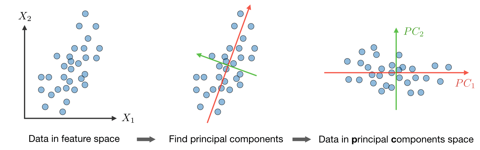
Principal component analysis
It is a dimension reduction technique that finds the variance maximizing directions onto which to project the data.
- Eigenvalue, eigenvector: Given a matrix \(A\in\mathbb{R}^{n\times n}\), \(\lambda\) is said to be an eigenvalue of \(A\) if there exists a vector \(z\in\mathbb{R}^n\backslash\{0\}\), called eigenvector, such that we have:
\[ \boxed{Az=\lambda z} \]
- Spectral theorem: Let \(A\in\mathbb{R}^{n\times n}\). If \(A\) is symmetric, then \(A\) is diagonalizable by a real orthogonal matrix \(U\in\mathbb{R}^{n\times n}\). By noting \(\Lambda=\textrm{diag}(\lambda_1,...,\lambda_n)\), we have:
\[ \boxed{\exists\Lambda\textrm{ diagonal},\quad A=U\Lambda U^T} \]
Remark: the eigenvector associated with the largest eigenvalue is called principal eigenvector of matrix \(A\).
Algorithm: The Principal Component Analysis (PCA) procedure is a dimension reduction technique that projects the data on \(k\) dimensions by maximizing the variance of the data as follows:
Step 1: Normalize the data to have a mean of 0 and standard deviation of 1. \[ \boxed{ \begin{align} x_j^{(i)}&\leftarrow\frac{x_j^{(i)}-\mu_j}{\sigma_j}\\ \mu_j &= \frac{1}{m}\sum_{i=1}^mx_j^{(i)}\\ \sigma_j^2&=\frac{1}{m}\sum_{i=1}^m(x_j^{(i)}-\mu_j)^2 \end{align} } \]
Step 2: Compute \(\displaystyle\Sigma=\frac{1}{m}\sum_{i=1}^mx^{(i)}{x^{(i)}}^T\in\mathbb{R}^{n\times n}\), which is symmetric with real eigenvalues.
Step 3: Compute \(u_1, ..., u_k\in\mathbb{R}^n\) the \(k\) orthogonal principal eigenvectors of \(\Sigma\), i.e. the orthogonal eigenvectors of the \(k\) largest eigenvalues.
Step 4: Project the data on \(\textrm{span}_\mathbb{R}(u_1,...,u_k)\).
This procedure maximizes the variance among all \(k\)-dimensional spaces.
Independent component analysis
It is a technique meant to find the underlying generating sources.
- Assumptions: We assume that our data \(x\) has been generated by the \(n\)-dimensional source vector \(s=(s_1,...,s_n)\), where \(s_i\) are independent random variables, via a mixing and non-singular matrix \(A\) as follows:
\[ \boxed{x=As} \]
The goal is to find the unmixing matrix \(W=A^{-1}\).
Bell and Sejnowski ICA algorithmThis algorithm finds the unmixing matrix \(W\) by following the steps below:
Write the probability of \(x=As=W^{-1}s\) as: \[ p(x)=\prod_{i=1}^np_s(w_i^Tx)\cdot|W| \]
Write the log likelihood given our training data \(\{x^{(i)}, i\in[\![1,m]\!]\}\) and by noting \(g\) the sigmoid function as: \[ l(W)=\sum_{i=1}^m\left(\sum_{j=1}^n\log\Big(g'(w_j^Tx^{(i)})\Big)+\log|W|\right) \]
Therefore, the stochastic gradient ascent learning rule is such that for each training example \(x^{(i)}\), we update \(W\) as follows: \[ \boxed{W\longleftarrow W+\alpha\left(\begin{pmatrix}1-2g(w_1^Tx^{(i)})\\1-2g(w_2^Tx^{(i)})\\\vdots\\1-2g(w_n^Tx^{(i)})\end{pmatrix}{x^{(i)}}^T+(W^T)^{-1}\right)} \]
