Supervised Learning cheatsheet
By Afshine Amidi and Shervine Amidi
Introduction to Supervised Learning
Given a set of data points \(\{x^{(1)}, ..., x^{(m)}\}\) associated to a set of outcomes \(\{y^{(1)}, ..., y^{(m)}\}\), we want to build a classifier that learns how to predict \(y\) from \(x\).
- Type of prediction: The different types of predictive models are summed up in the table below:
| Regression | Classifier | |
|---|---|---|
| Outcome | Continuous | Class |
| Examples | Linear regression | Logistic regression, SVM, Naive Bayes |
- Type of model: The different models are summed up in the table below:
| Discriminative model | Generative model | |
|---|---|---|
| Goal | Directly estimate \(P(x|y)\) | Estimate \(P(x|y)\) to then deduce \(P(y|x)\) |
| What's learned | Decision boundary | Probability distributions of the data |
| Illustration | 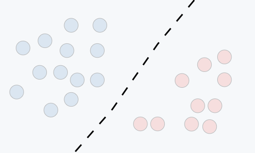 |
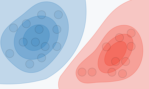 |
| Examples | Regressions, SVMs | GDA, Naive Bayes |
Notations and general concepts
- Hypothesis: The hypothesis is noted \(h_\theta\) and is the model that we choose. For a given input data \(x^{(i)}\) the model prediction output is \(h_\theta(x^{(i)})\).
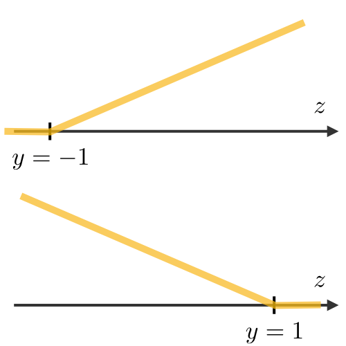
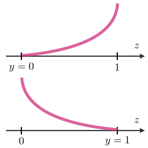
- Loss function: A loss function is a function \(L:(z,y)\in\mathbb{R}\times Y\longmapsto L(z,y)\in\mathbb{R}\) that takes as inputs the predicted value \(z\) corresponding to the real data value \(y\) and outputs how different they are. The common loss functions are summed up in the table below:
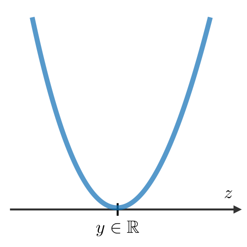
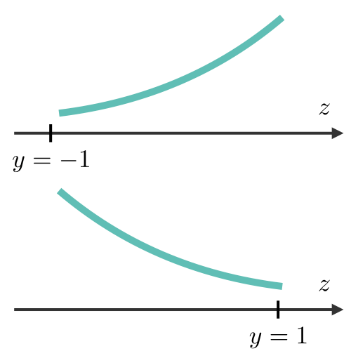
| Least squared error | Logistic loss | Hinge loss | Cross-entropy |
|---|---|---|---|
| \(\quad \displaystyle\frac{1}{2}(y-z)^2 \quad\) | \(\displaystyle\log(1+\exp(-yz))\) | \(\max(0,1-yz)\) | \((y-1)\log(1-z)\) \(-y\log(z)\) |
 |
 |
 |
 |
| Linear regression | Logistic regression | SVM | Neural |
- Cost function: The cost function \(J\) is commonly used to assess the performance of a model, and is defined with the loss function \(L\) as follows:
\[ \boxed{J(\theta)=\sum_{i=1}^mL(h_\theta(x^{(i)}), y^{(i)})} \]
- Gradient descent: By noting \(\alpha\in\mathbb{R}\) the learning rate, the update rule for gradient descent is expressed with the learning rate and the cost function \(J\) as follows:
\[ \boxed{\theta\longleftarrow\theta-\alpha\nabla J(\theta)} \]
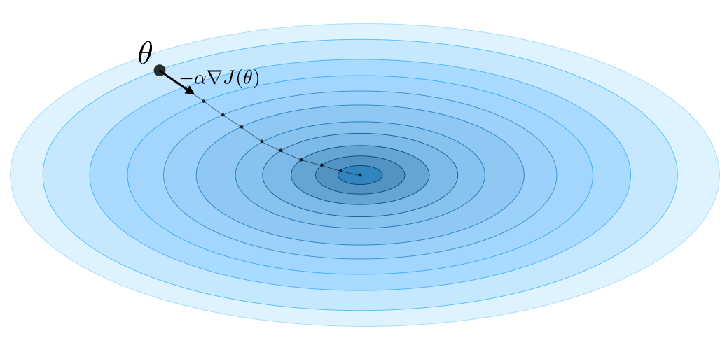
Remark: Stochastic gradient descent (SGD) is updating the parameter based on each training example, and batch gradient descent is on a batch of training examples.
- Likelihood: The likelihood of a model \(L(\theta)\) given parameters \(\theta\) is used to find the optimal parameters \(\theta\) through maximizing the likelihood. In practice, we use the log-likelihood \(\ell(\theta)=\log(L(\theta))\) which is easier to optimize. We have:
\[ \boxed{\theta^{\textrm{opt}}=\underset{\theta}{\textrm{arg max }}L(\theta)} \]
- Newton's algorithm: The Newton's algorithm is a numerical method that finds \(\theta\) such that \(\ell'(\theta)=0\). Its update rule is as follows:
\[ \boxed{\theta\leftarrow\theta-\frac{\ell'(\theta)}{\ell^{\prime\prime}(\theta)}} \]
Remark: the multidimensional generalization, also known as the Newton-Raphson method, has the following update rule: \[ \theta\leftarrow\theta-\left(\nabla_\theta^2\ell(\theta)\right)^{-1}\nabla_\theta\ell(\theta) \]
Linear models
Linear regression
We assume here that \(y|x;\theta\sim\mathcal{N}(\mu,\sigma^2)\)
- Normal equations: By noting \(X\) the design matrix, the value of \(\theta\) that minimizes the cost function is a closed-form solution such that:
\[ \boxed{\theta=(X^TX)^{-1}X^Ty} \]
- LMS algorithm: By noting \(\alpha\) the learning rate, the update rule of the Least Mean Squares (LMS) algorithm for a training set of \(m\) data points, which is also known as the Widrow-Hoff learning rule, is as follows:
\[ \boxed{\forall j,\quad \theta_j \leftarrow \theta_j+\alpha\sum_{i=1}^m\left[y^{(i)}-h_\theta(x^{(i)})\right]x_j^{(i)}} \]
Remark: the update rule is a particular case of the gradient ascent.
- LWR: a variant of linear regression that weights each training example in its cost function by \(w^{(i)}(x)\), which is defined with parameter \(\tau\in\mathbb{R}\) as:
\[ \boxed{w^{(i)}(x)=\exp\left(-\frac{(x^{(i)}-x)^2}{2\tau^2}\right)} \]
Classific ation and logistic regression
- Sigmoid function: The sigmoid function \(g\), also known as the logistic function, is defined as follows:
\[ \forall z\in\mathbb{R},\quad\boxed{g(z)=\frac{1}{1+e^{-z}}\in]0,1[} \]
- Softmax regression: A softmax regression, also called a multiclass logistic regression, is used to generalize logistic regression when there are more than 2 outcome classes. By convention, we set \(\theta_K=0\), which makes the Bernoulli parameter \(\phi_i\) of each class \(i\) equal to:
\[ \boxed{\displaystyle\phi_i=\frac{\exp(\theta_i^Tx)}{\displaystyle\sum_{j=1}^K\exp(\theta_j^Tx)}} \]
Generalized Linear Models
- Exponential family: A class of distributions is said to be in the exponential family if it can be written in terms of a natural parameter, also called the canonical parameter or link function, \(\eta\), a sufficient statistic \(T(y)\) and a log-partition function \(a(\eta)\) as follows:
\[ \boxed{p(y;\eta)=b(y)\exp(\eta T(y)-a(\eta))} \]
Remark: we will often have \(T(y)=y\). Also, \(\exp(-a(\eta))\) can be seen as a normalization parameter that will make sure that the probabilities sum to one.
Here are the most common exponential distributions summed up in the following table:
| Distribution | \(\eta\) | \(T(y)\) | \(a(\eta)\) | \(b(y)\) |
|---|---|---|---|---|
| Bernoulli | \(\log\left(\frac{\phi}{1-\phi}\right)\) | \(y\) | \(\log(1+\exp(\eta))\) | \(1\) |
| Gaussian | \(\mu\) | \(y\) | \(\frac{\eta^2}{2}\) | \(\frac{1}{\sqrt{2\pi}}\exp\left(-\frac{y^2}{2}\right)\) |
| Poisson | \(\log(\lambda)\) | \(y\) | \(e^{\eta}\) | \(\frac{1}{y!}\) |
| Geometric | \(\log(1-\phi)\) | \(y\) | \(\log\left(\frac{e^\eta}{1-e^\eta}\right)\) | \(1\) |
- Assumptions of GLMs: Generalized Linear Models (GLM) aim at predicting a random variable \(y\) as a function of \(x\in\mathbb{R}^{n+1}\) and rely on the following 3 assumptions:
- \((1)\quad\boxed{y|x;\theta\sim\textrm{ExpFamily}(\eta)}\)
- \((2)\quad\boxed{h_\theta(x)=E[y|x;\theta]}\)
- \((3)\quad\boxed{\eta=\theta^Tx}\)
Remark: ordinary least squares and logistic regression are special cases of generalized linear models.
Support Vector Machines
The goal of support vector machines is to find the line that maximizes the minimum distance to the line.
- Optimal margin classifier: The optimal margin classifier \(h\) is such that:
\[ \boxed{h(x)=\textrm{sign}(w^Tx-b)} \]
where \((w, b)\in\mathbb{R}^n\times\mathbb{R}\) is the solution of the following optimization problem: \[
\boxed{\min\frac{1}{2}\|w\|^2}\quad\quad\textrm{such that }\quad \boxed{y^{(i)}(w^Tx^{(i)}-b)\geqslant1}
\] 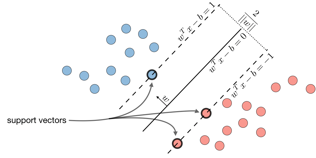
Remark: the line is defined as \(\boxed{w^Tx-b=0}\).
- Hinge loss: The hinge loss is used in the setting of SVMs and is defined as follows:
\[ \boxed{L(z,y)=[1-yz]_+=\max(0,1-yz)} \]
- Kernel: Given a feature mapping \(\phi\), we define the kernel \(K\) to be defined as:
\[ \boxed{K(x,z)=\phi(x)^T\phi(z)} \]
In practice, the kernel \(K\) defined by \(K(x,z)=\exp\left(-\frac{\|x-z\|^2}{2\sigma^2}\right)\) is called the Gaussian kernel and is commonly used.
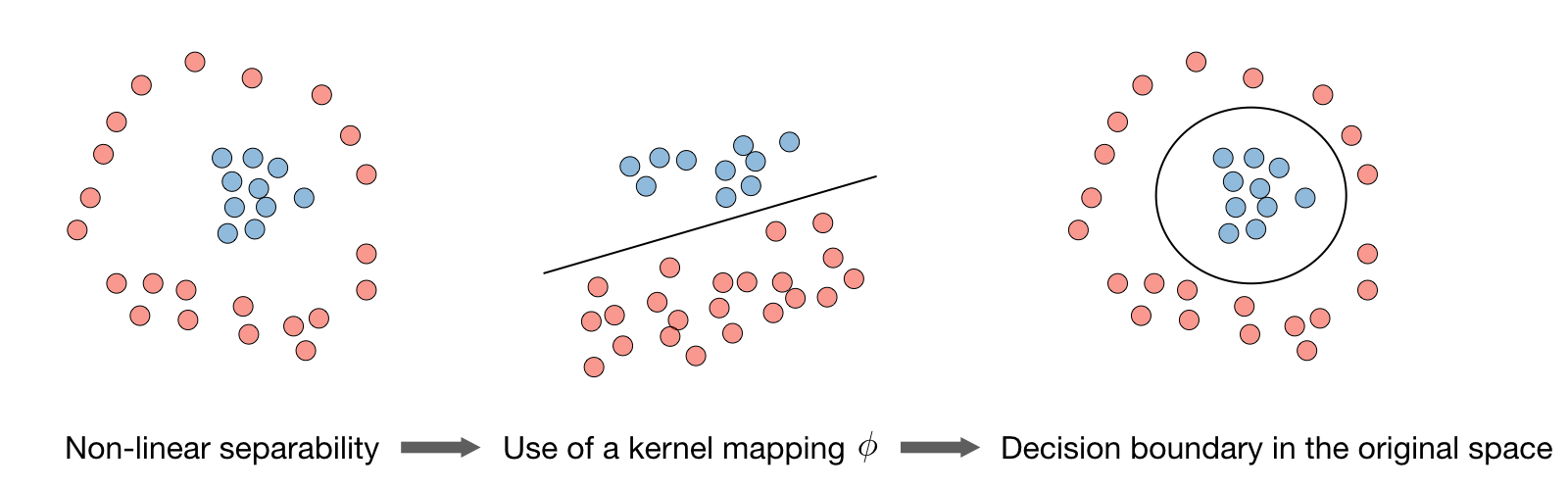
Remark: we say that we use the "kernel trick" to compute the cost function using the kernel because we actually don't need to know the explicit mapping \(\phi\), which is often very complicated. Instead, only the values \(K(x,z)\) are needed.
- Lagrangian: We define the Lagrangian \(\mathcal{L}(w,b)\) as follows:
\[ \boxed{\mathcal{L}(w,b)=f(w)+\sum_{i=1}^l\beta_ih_i(w)} \]
Remark: the coefficients \(\beta_i\) are called the Lagrange multipliers.
Generative Learning
A generative model first tries to learn how the data is generated by estimating \(P(x|y)\), which we can then use to estimate \(P(y|x)\) by using Bayes' rule.
Gaussian Discriminant Analysis
- Setting:The Gaussian Discriminant Analysis assumes that \(y\) and \(x|y=0\) and \(x|y=1\) are such that:
- \((1)\quad\boxed{y\sim\textrm{Bernoulli}(\phi)}\)
- \((2)\quad\boxed{x|y=0\sim\mathcal{N}(\mu_0,\Sigma)}\)
- \((3)\quad\boxed{x|y=1\sim\mathcal{N}(\mu_1,\Sigma)}\)
- Estimation: The following table sums up the estimates that we find when maximizing the likelihood:
| \(\widehat{\phi}\) | \(\displaystyle\frac{1}{m}\sum_{i=1}^m1_{(y^{(i)}=1)}\) |
|---|---|
| \(\widehat{\mu_j}\quad{\small(j=0,1)}\) | \(\displaystyle\frac{\sum_{i=1}^m1_{(y^{(i)}=j)}x^{(i)}}{\sum_{i=1}^m1_{(y^{(i)}=j)}}\) |
| \(\widehat{\Sigma}\) | \(\displaystyle\frac{1}{m}\sum_{i=1}^m(x^{(i)}-\mu_{y^{(i)}})(x^{(i)}-\mu_{y^{(i)}})^T\) |
Naive Bayes
- Assumption: The Naive Bayes model supposes that the features of each data point are all independent:
\[ \boxed{P(x|y)=P(x_1,x_2,...|y)=P(x_1|y)P(x_2|y)...=\prod_{i=1}^nP(x_i|y)} \]
- Solutions: Maximizing the log-likelihood gives the following solutions, with \(k\in\{0,1\},l\in[\![1,L]\!]\)
\[ \boxed{ \begin{align} P(y=k)&=\frac{1}{m}\times\#\{j|y^{(j)}=k\}\\ P(x_i=l|y=k)&=\frac{\#\{j|y^{(j)}=k\textrm{ and }x_i^{(j)}=l\}}{\#\{j|y^{(j)}=k\}} \end{align} } \]
Remark: Naive Bayes is widely used for text classification and spam detection.
Tree-based and ensemble methods
These methods can be used for both regression and classification problems.
CART: Classification and Regression Trees (CART), commonly known as decision trees, can be represented as binary trees. They have the advantage to be very interpretable.
Random forest: It is a tree-based technique that uses a high number of decision trees built out of randomly selected sets of features. Contrary to the simple decision tree, it is highly uninterpretable but its generally good performance makes it a popular algorithm.
Remark: random forests are a type of ensemble methods.
- Boosting: The idea of boosting methods is to combine several weak learners to form a stronger one. The main ones are summed up in the table below:
| Adaptive boosting | Gradient boosting |
|---|---|
| • Known as Adaboost • High weights are put on errors to improve at the next boosting step |
• Weak learners trained on remaining errors |
Other non-parametric approaches
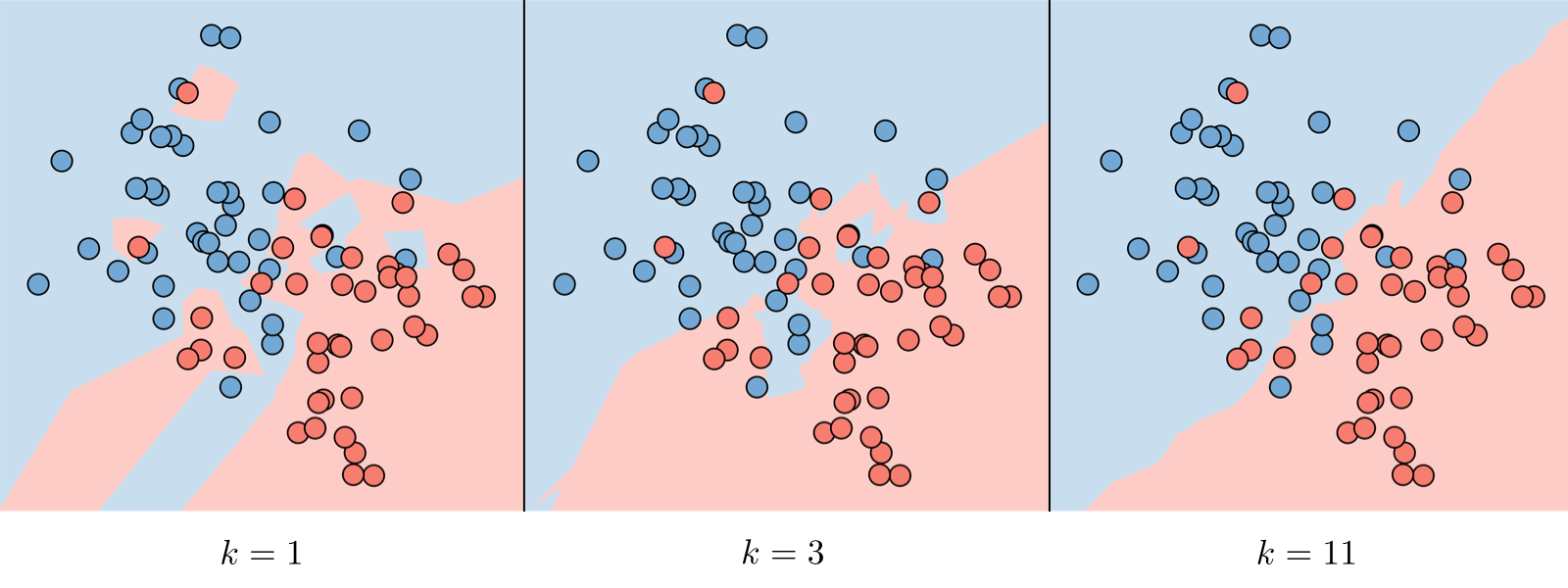
- \(k\)-nearest neighbors: The \(k\)-nearest neighbors algorithm, commonly known as \(k\)-NN, is a non-parametric approach where the response of a data point is determined by the nature of its \(k\) neighbors from the training set. It can be used in both classification and regression settings.
Remark: The higher the parameter \(k\), the higher the bias, and the lower the parameter \(k\), the higher the variance.
Learning Theory
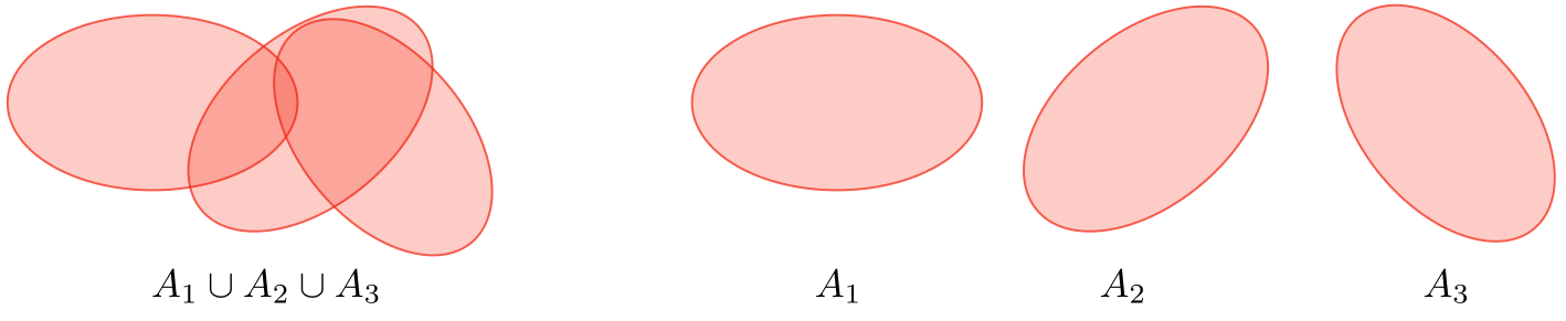
- Union boundLet \(A_1, ..., A_k\) be \(k\) events. We have:
\[ \boxed{P(A_1\cup ...\cup A_k)\leqslant P(A_1)+...+P(A_k)} \]
- Hoeffding inequality: Let \(Z_1, .., Z_m\) be \(m\) iid variables drawn from a Bernoulli distribution of parameter \(\phi\). Let \(\widehat{\phi}\) be their sample mean and \(\gamma>0\) fixed. We have:
\[ \boxed{P(|\phi-\widehat{\phi}|>\gamma)\leqslant2\exp(-2\gamma^2m)} \]
Remark: this inequality is also known as the Chernoff bound.
- Training error: For a given classifier \(h\), we define the training error \(\widehat{\epsilon}(h)\), also known as the empirical risk or empirical error, to be as follows:
\[ \boxed{\widehat{\epsilon}(h)=\frac{1}{m}\sum_{i=1}^m1_{(h(x^{(i)})\neq y^{(i)})}} \]
- Probably Approximately Correct (PAC): PAC is a framework under which numerous results on learning theory were proved, and has the following set of assumptions:
- the training and testing sets follow the same distribution
- the training examples are drawn independently
- Shattering: Given a set \(S=\{x^{(1)},...,x^{(d)}\}\), and a set of classifiers \(\mathcal{H}\), we say that \(\mathcal{H}\) shatters \(S\) if for any set of labels \(\{y^{(1)}, ..., y^{(d)}\}\), we have:
\[ \boxed{\exists h\in\mathcal{H}, \quad \forall i\in[\![1,d]\!],\quad h(x^{(i)})=y^{(i)}} \]
- Upper bound theorem: Let \(\mathcal{H}\) be a finite hypothesis class such that \(|\mathcal{H}|=k\) and let \(\delta\) and the sample size \(m\) be fixed. Then, with probability of at least \(1-\delta\), we have:
\[ \boxed{\epsilon(\widehat{h})\leqslant\left(\min_{h\in\mathcal{H}}\epsilon(h)\right)+2\sqrt{\frac{1}{2m}\log\left(\frac{2k}{\delta}\right)}} \]
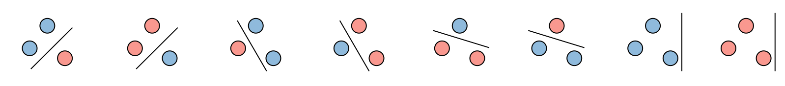
- VC dimension: The Vapnik-Chervonenkis (VC) dimension of a given infinite hypothesis class \(\mathcal{H}\), noted \(\textrm{VC}(\mathcal{H})\) is the size of the largest set that is shattered by \(\mathcal{H}\).
Remark: the VC dimension of \({\small\mathcal{H}=\{\textrm{set of linear classifiers in 2 dimensions}\}}\) is 3.
- Theorem (Vapnik): Let \(\mathcal{H}\) be given, with \(\textrm{VC}(\mathcal{H})=d\) and \(m\) the number of training examples. With probability at least \(1-\delta\), we have:
\[ \boxed{\epsilon(\widehat{h})\leqslant \left(\min_{h\in\mathcal{H}}\epsilon(h)\right) + O\left(\sqrt{\frac{d}{m}\log\left(\frac{m}{d}\right)+\frac{1}{m}\log\left(\frac{1}{\delta}\right)}\right)} \]
